Chapter 3 Hierarchical Modeling
3.1 Set Up
Creating a testing set
Since we have time-series data, we created a testing set by sub-setting each company’s 2nd to latest year. We left off the most recent year a company reports their earnings and created a testing set with this data, the training set includes all the other previous years. We will predict the earnings next year for each company with the testing set and compare it with the actual values to help determine model accuracy.
testing <- data_elimatedO %>%
   group_by(COMPANY) %>%
   filter(row_number()==1)

training <- anti_join(data_elimatedO, testing)
Tuning Priors
Earnings, like most things in the financial markets are quite volatile, making them harder to model. We do not have a strong understanding of the variability between and within companies, thus we are using weakly informative priors. This means that the models will rely more on the data to form the posterior distributions. We are using the default prior values found in the stan_glmer package.
Defining Notation
In our model notation below, \(Y_{ij}\) is earnings for the next year after the \(i\)th year for company \(j\) and \(X_{ij}\) is the earnings in the \(i\)th year for company \(j\). For example, Y = Earnings of Apple in 2017 in billions, and X = Earnings of Apple in 2016 in billions.
3.2 Model 1: Hierarchical w/ Different Intercepts
3.2.1 Model Structure
Now, we will move on to utilizing the structure of our data, where we have consecutive observations for each company for several years. We start with a model with varying intercepts. Note: we fit each model using training data for evaluation purposes.
Diff_inter_train <- readRDS("Diff_inter_train_nick.rds")model_diff_inter_train_data <- training %>%
select(c("Earnings_next_year_Scaled","EARNINGS_Scaled","EARNINGS_1_YEAR_AGO","COMPANY","Sector")) %>% na.omit()
model_diff_inter_train <- stan_glmer(
Earnings_next_year_Scaled ~ EARNINGS_Scaled + EARNINGS_1_YEAR_AGO + Sector + (1 | COMPANY) , data = model_diff_inter_train_data,
family = gaussian,
chains = 4, iter = 5000*2, seed = 84735,
prior_PD = FALSE, refresh = 0)
write_rds(model_diff_inter_train, "Diff_Inter_train_nick.rds")prior_summary(Diff_inter_train)Below is the notation for the differing intercepts model:
\[\begin{split} \text{Relationship within company:} & \\ Y_{ij} | \beta_{0j}, \beta_1, \sigma_y & \sim N(\mu_{ij}, \sigma_y^2) \;\; \text{ where } \mu_{ij} = \beta_{0j} + \beta_1 X_{ij} + \beta_2 X_{ij} + \beta_3 X_{ij}...\\ & \\ \text{Variability between companies:} & \\ \beta_{0j} & \stackrel{ind}{\sim} N(\beta_0, \sigma_0^2) \\ & \\ \text{Prior information on Globals with Adjusted Prior} & \\ \beta_{0c} & \sim N(0.59, 1.5^2) \\ \beta_1 & \sim N(0, 1.74^2) \\ \beta_2 & \sim N(0, 1.60^2) \\ \beta_3 & \sim N(0, 4.60^2) \\ .\\ .\\ .\\ \sigma_y & \sim \text{Exp}(1.6) \\ \sigma_0 & \sim \text{Exp}(1) \\ \end{split}\]
3.3 Model 2: Hierarchical w/ Different Slopes and Intercepts
3.3.1 Model Structure
In addition to having a hierarchical regression with different intercepts, we decided to add a model with different intercepts and slopes.
Rational behind different slopes:
Below we graph 4 random companies, we can see that earnings in the current year impacts earnings next year differently among different companies.
eliminated %>%
  filter(COMPANY %in% c("AAL","CVS","DAL","WAB")) %>%
  ggplot(., aes(x = EARNINGS_Scaled, y = Earnings_next_year_Scaled)) +
    geom_point() +
    geom_smooth(method = "lm", se = FALSE) +
    facet_grid(~ COMPANY)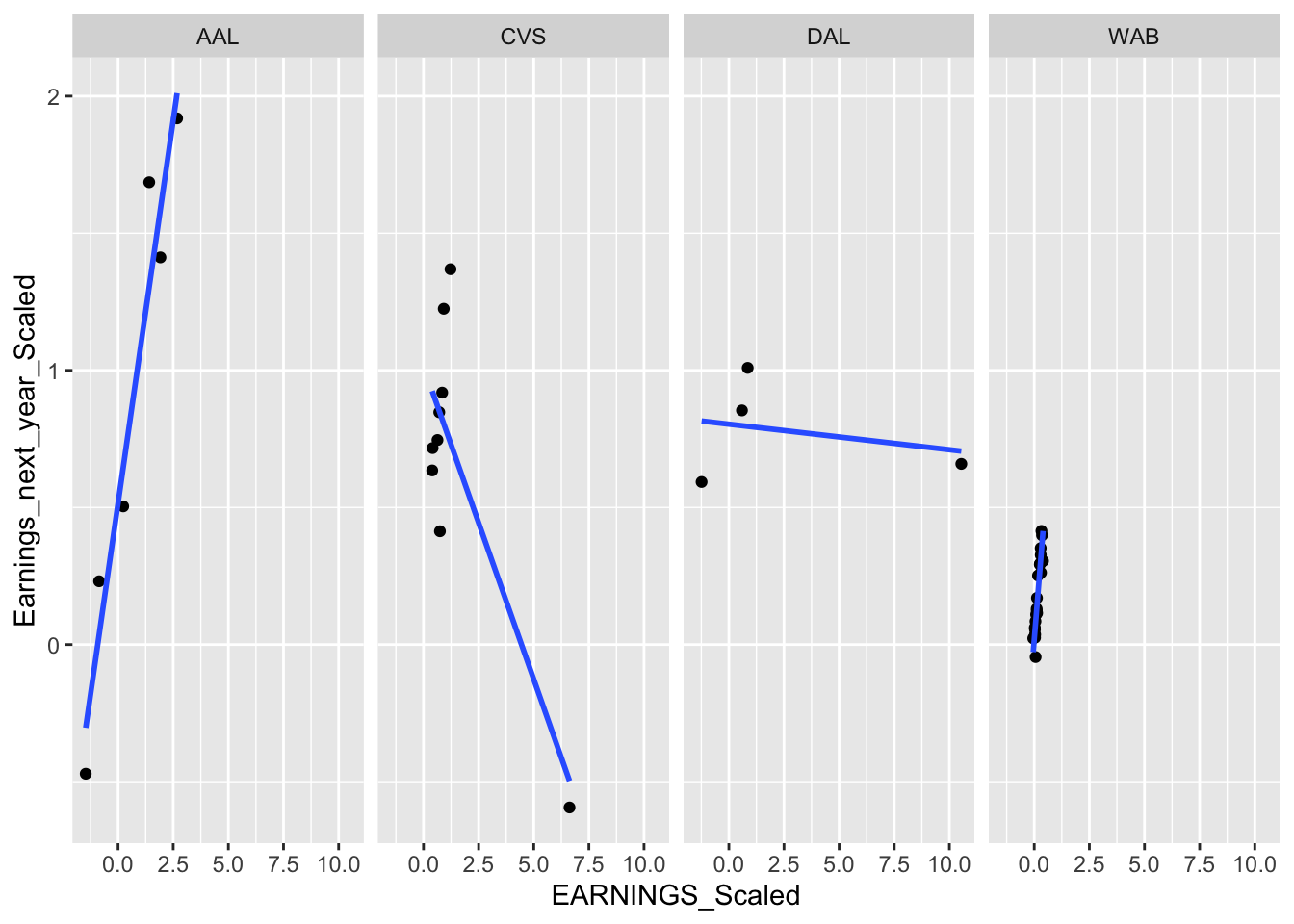
To get a better idea of the varying slopes, we graphed 50 random companies together.
vector <- eliminated$COMPANY
vector <- sample_n(as.data.frame(vector), 50)
vector <- as.list(vector)
eliminated %>%
  filter(COMPANY %in% vector$vector) %>%
  ggplot(aes(x=EARNINGS_Scaled, y= Earnings_next_year_Scaled, group = COMPANY))+
  geom_smooth(method = "lm", se= FALSE, size = 0.5)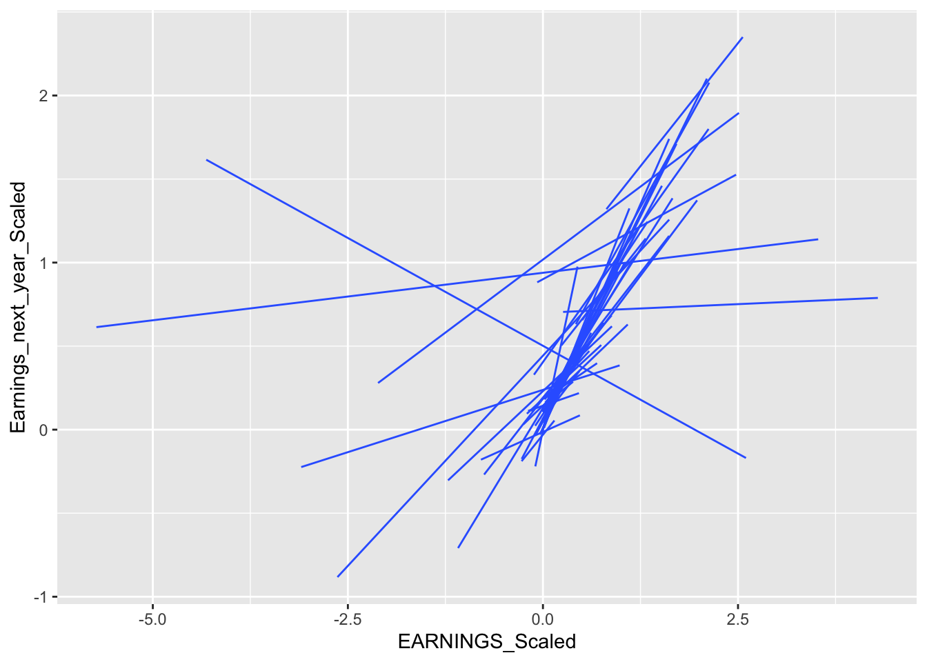
Instead of using a global earnings slope coefficient, we decide to add a hierarchical layer so that company slope coefficients can learn from each other and yet have their own specific slope. If we have a universal slope coefficient, there will be a great deal of bias within our model.
Diff_inter_slope_train <- readRDS("Diff_inter_slope_train_nick.rds")model_diff_inter_slope_train_data <- training %>%
select(c("Earnings_next_year_Scaled","Sector","COMPANY","EARNINGS_Scaled","EARNINGS_1_YEAR_AGO")) %>%
na.omit()
diff_slope_inter_model_train <- stan_glmer(
Earnings_next_year_Scaled ~ EARNINGS_Scaled + EARNINGS_1_YEAR_AGO + (EARNINGS_Scaled | COMPANY) + Sector, data = model_diff_inter_slope_train_data,
family = gaussian,
chains = 4, iter = 5000*2, seed = 84735,
prior_PD = FALSE)
write_rds(diff_slope_inter_model_train, "Diff_inter_slope_train_nick.rds")prior_summary(Diff_inter_slope_train)Different intercepts & slopes model notation:
\[\begin{split} Y_{ij} | \beta_{0j}, \beta_{1j}, \sigma_y & \sim N(\mu_{ij}, \sigma_y^2) \;\; \text{ where } \; \mu_{ij} = \beta_{0j} + \beta_{1j} X_{ij} + \beta_{2} X_{ij} + \beta_{3} X_{ij}...\\ & \\ \beta_{0j} & \sim N(\beta_0, \sigma_0^2) \\ \beta_{1j} & \sim N(\beta_1, \sigma_1^2) \\ & \\ \beta_{0c} & \sim N(0.59, 1.5^2) \\ \beta_1 & \sim N(0, 1.74^2) \\ .\\ .\\ .\\ \sigma_y & \sim \text{Exp}(1.6) \\ \sigma_0, \sigma_1, ... & \sim \text{(something a bit complicated)}. \\ \end{split}\]
3.4 Model Evaluations
3.4.1 Is this the right model?
Using our models we simulate replicated data and then compare these to the observed data to look for discrepancies between the two in the plots below.
pp_check(Diff_inter_train) 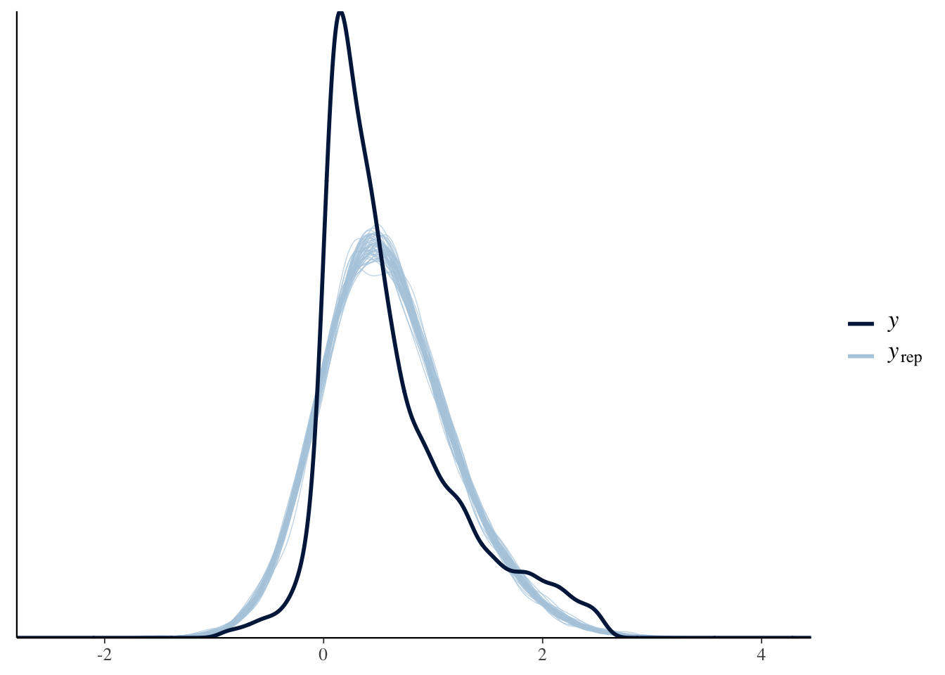
pp_check(Diff_inter_slope_train)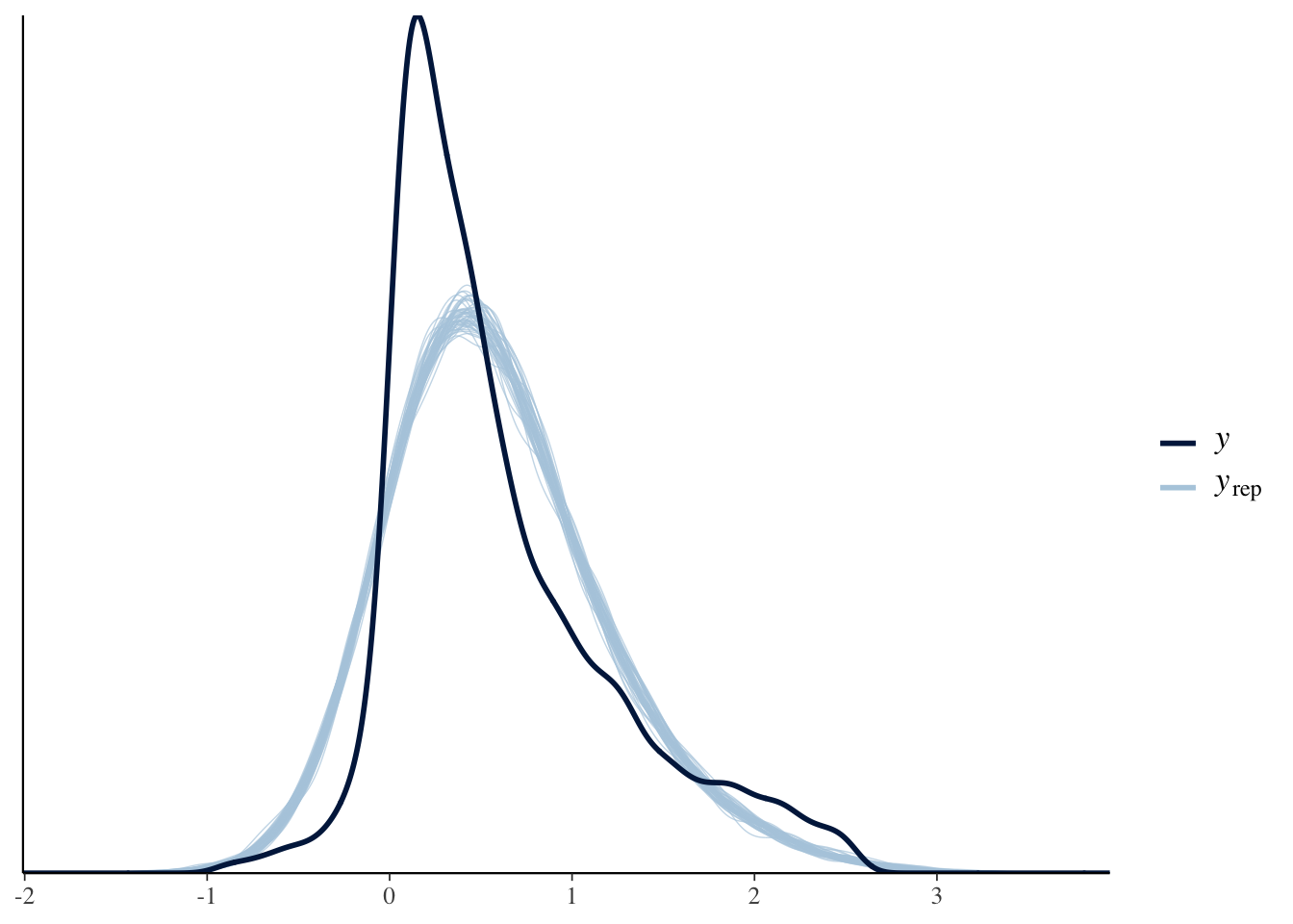
Several company earnings’ on the right seem to be causing model fitness difficulties. Both models run into this problem, however the second model is able to capture more of the outliers on the right.
Prior to removing the extreme outliers in our data set, the posterior predictive check for the models were worse as it left majority of the outliers uncovered. After filtering out for outliers, we evidently still have problems with both models.
Next we will examine the predictive accuracy of the models.
3.4.2 How Accurate are the models?
Below, we compare our predictions for American Airlines, Delta Airlines, and Amazon. We plot 750 random values predicted from our predictions (out of 20,000) for both models. We can see below our predictions for each of these companies for both hierarchical models.
Model 1 - Specific Examples with companies:
set.seed(84732)
predict_model("AAL", Diff_inter_train)
set.seed(84732)
predict_model("DAL", Diff_inter_train)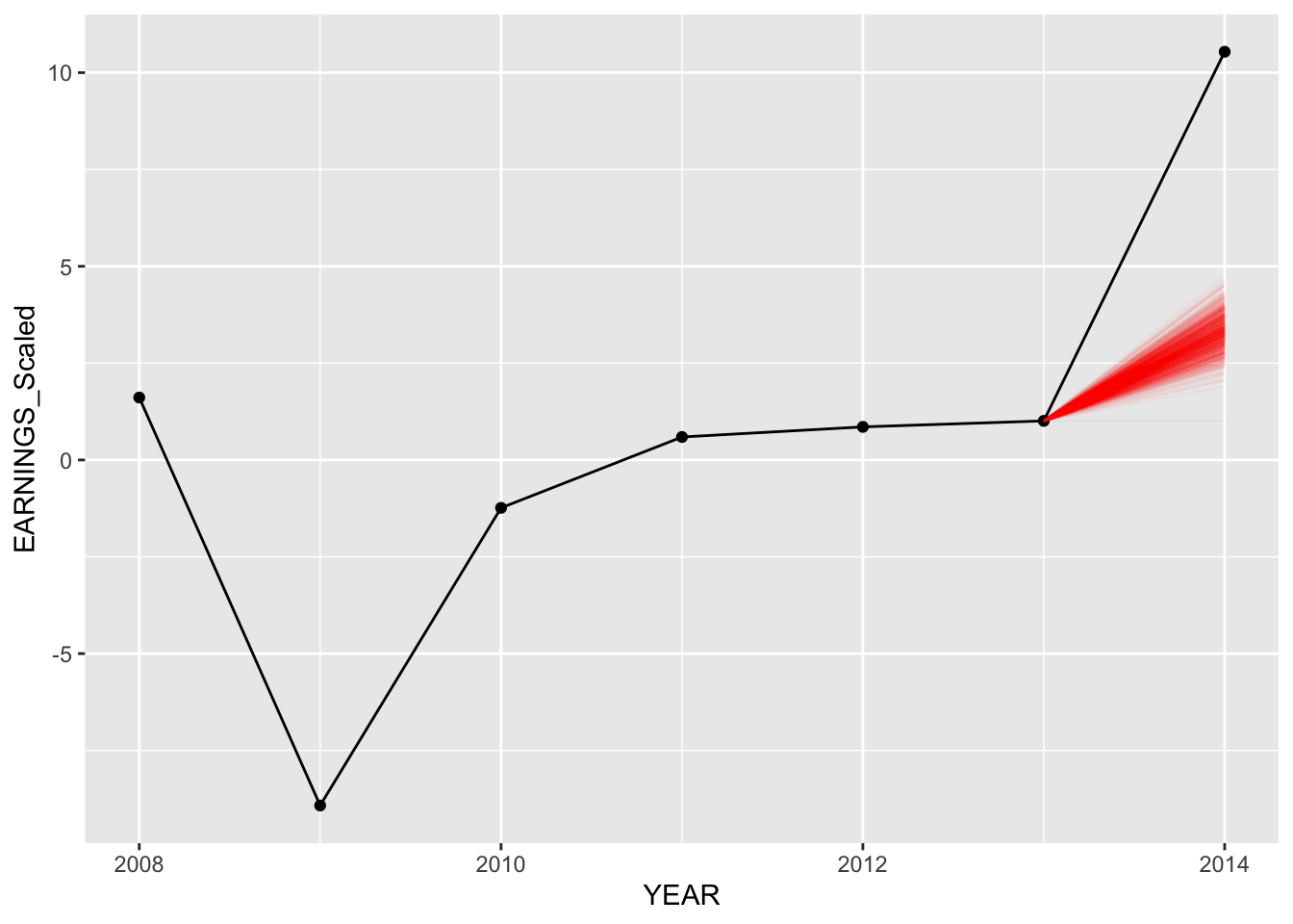
set.seed(84732)
predict_model("AMZN", Diff_inter_train)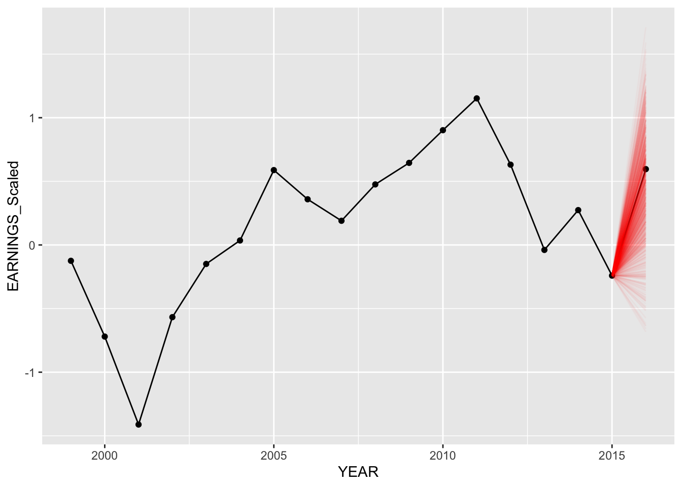
Model 2 - Specific Examples with companies:
set.seed(84732)
predict_model("AAL", Diff_inter_slope_train)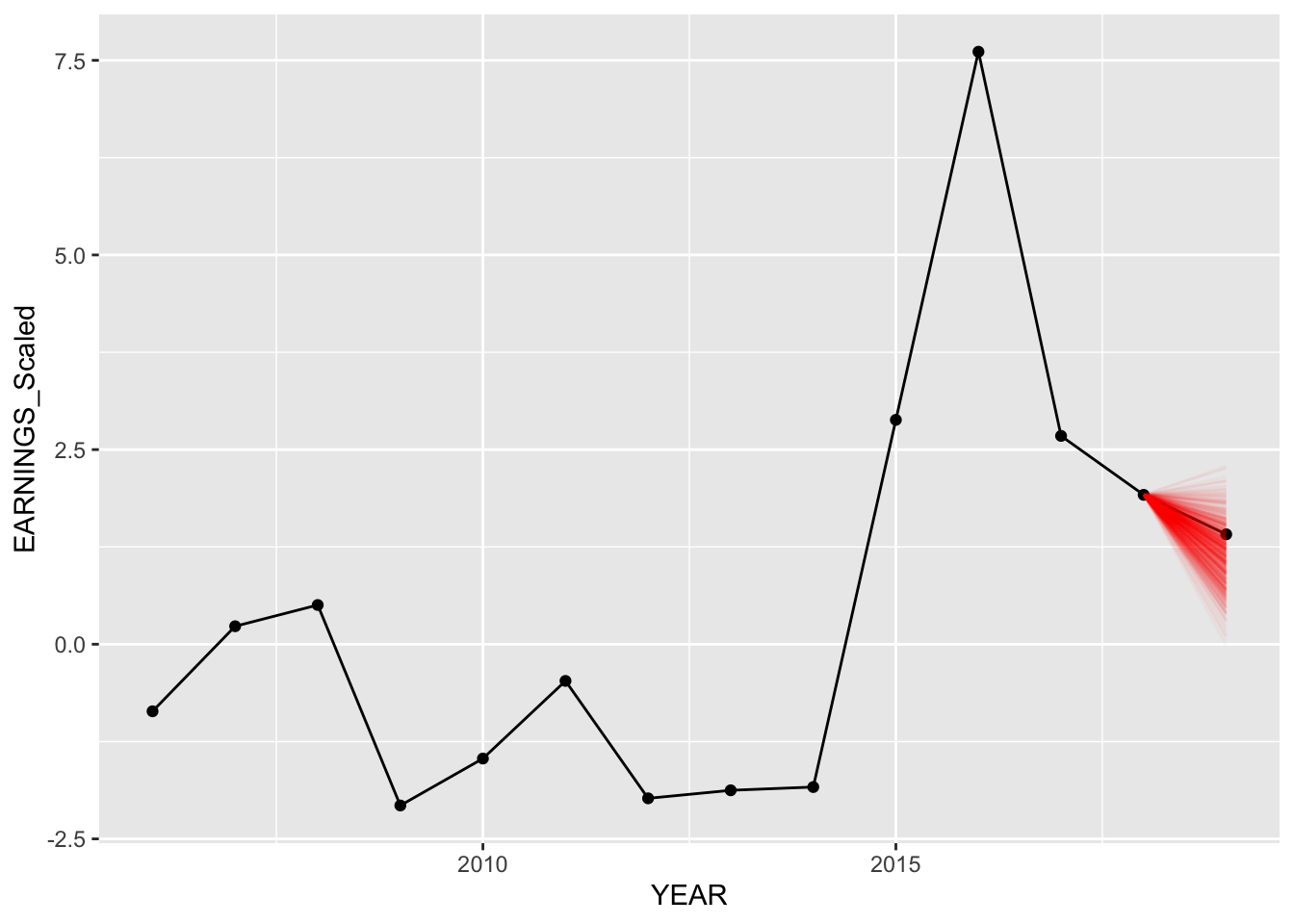
set.seed(84732)
predict_model("DAL", Diff_inter_slope_train)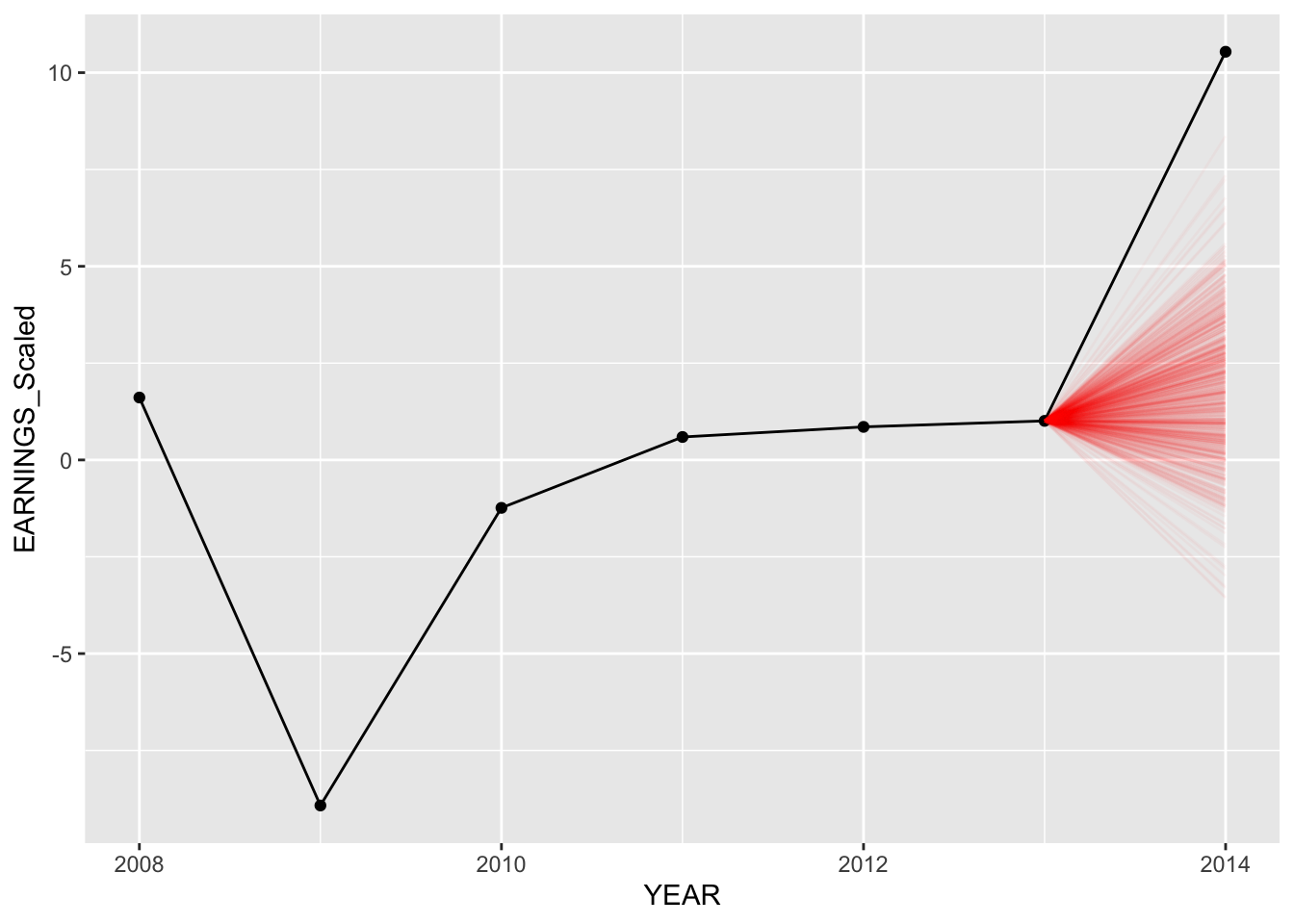
set.seed(84732)
predict_model("AMZN", Diff_inter_slope_train)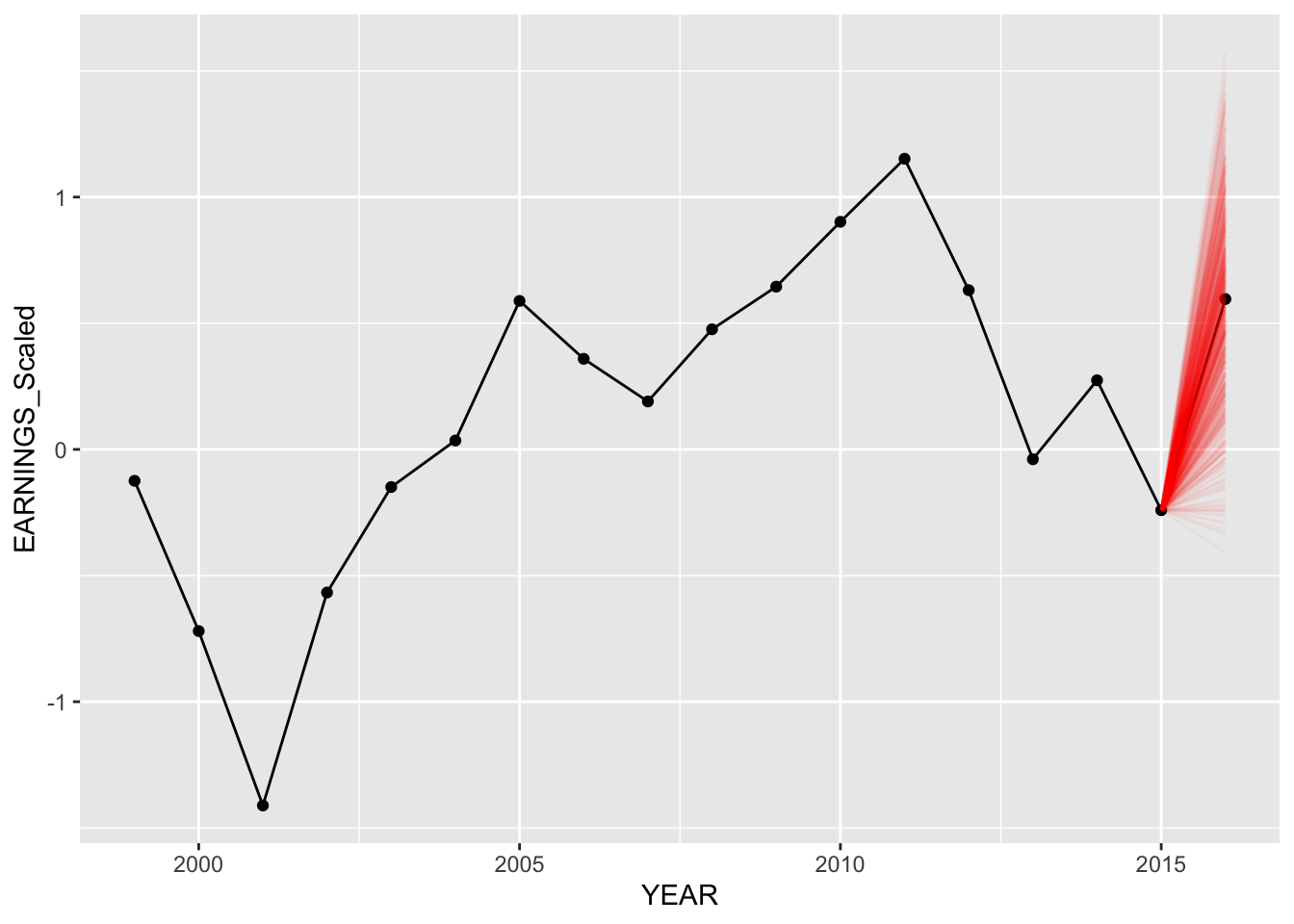
The predictions for the second model (different intercepts and slopes) seem to be slightly better as more posterior predictive points are nearer to the actual values of earnings in “2020”.
Notice how for both models, predictions for Delta Air Lines are completely off from the actual data. However, in our model with different intercepts and slopes, more predictions are closer to the actual value, thus having the model mean being closer as well.
Evaluating Metrics
For the prediction metrics, using the training data set, we calculated 20,000 values for each individual company for their earnings next year (the last year we have data on them) using the hierarchical models. We then take the median value of the 20,000 for each company and calculate the mean distance from the median to the actual earnings observed for that year. We also computed the 95% and 50% prediction intervals by calculating the percentage of 20,000 predicted values are within the 2.5th and 97.5th percentile and 25 to 75th percentile respectively.
Different Intercepts Model:
Diff_inter_metrics## MAE Within95 Within50 Within90
## 1 0.3620034 0.7543103 0.4181034 0.7090517Different Intercepts & Slopes Model:
Diff_inter_slope_metrics## MAE Within95 Within50 Within90
## 1 0.2781092 0.7931034 0.4935345 0.7262931We can see that our model with varying intercepts and slopes (model 2) preforms slightly better. Where our average median posterior prediction is off by 0.28 billion as opposed to 0.362 billion when we only have differing intercepts. Furthermore, our 95 and 50 interval values are both better in the model with different intercept and slope.
Shrinkage
Since we modeled based off different companies having different intercepts, it is worthwhile to checkout how the company baselines shrunk compared to each other and between the two different models. We randomly sampled 70 companies, since if we plot all companies we will have more than 400 companies on the X-axis. We can visually see how the intercepts become less varied as we are looking at the hierarchical model with different intercept and slopes.
Model 1 Shrinkage:
set.seed(84732)
COMPANY_chains <- Diff_inter_train %>%
  spread_draws(`(Intercept)`, b[,COMPANY]) %>%
  mutate(mu_j = `(Intercept)` + b)
COMPANY_summary_scaled <- COMPANY_chains %>%
  select(-`(Intercept)`, -b) %>%
  mean_qi(.width = 0.80) %>%
  mutate(COMPANY = fct_reorder(COMPANY, mu_j))
ggplot(
    sample_n(COMPANY_summary_scaled,70),
    aes(x = COMPANY, y = mu_j, ymin = .lower, ymax = .upper)) +
    geom_pointrange() +
    geom_hline(yintercept = mean(data$Earnings_next_year_Scaled), linetype = "dashed") +
  xaxis_text(angle = 90, hjust = 1)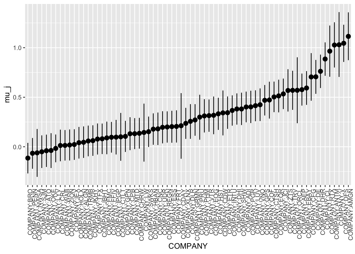
Model 2 Shrinkage:
set.seed(84732)
COMPANY_chains <- Diff_inter_slope_train %>%
  spread_draws(`(Intercept)`, b[,COMPANY]) %>%
  mutate(mu_j = `(Intercept)` + b)
COMPANY_summary_scaled <- COMPANY_chains %>%
  select(-`(Intercept)`, -b) %>%
  mean_qi(.width = 0.80) %>%
  mutate(COMPANY = fct_reorder(COMPANY, mu_j))
ggplot(
    sample_n(COMPANY_summary_scaled,70),
    aes(x = COMPANY, y = mu_j, ymin = .lower, ymax = .upper)) +
    geom_pointrange() +
    geom_hline(yintercept = mean(data$Earnings_next_year_Scaled), linetype = "dashed") +
  xaxis_text(angle = 90, hjust = 1)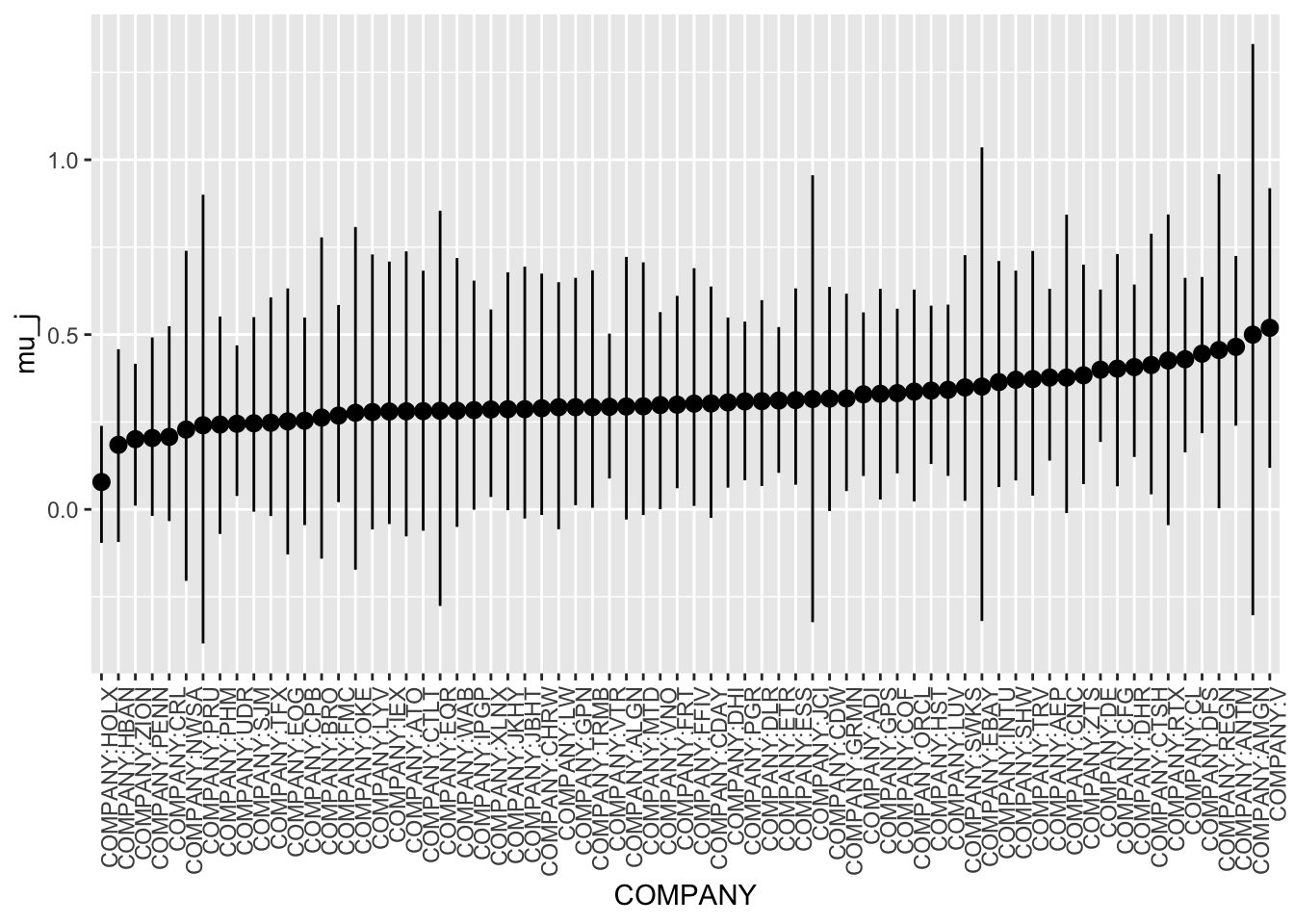
3.4.3 Interpreting Coefficents
tidy(Diff_inter_train, effects = "fixed", conf.int = TRUE, conf.level = .80)## # A tibble: 13 × 5
## term estimate std.error conf.low conf.high
## <chr> <dbl> <dbl> <dbl> <dbl>
## 1 (Intercept) 0.320 0.0744 0.225 0.417
## 2 EARNINGS_Scaled 0.222 0.00686 0.213 0.230
## 3 EARNINGS_1_YEAR_AGO 0.0961 0.00613 0.0883 0.104
## 4 SectorConsumer Discretionary 0.115 0.0856 0.00449 0.225
## 5 SectorConsumer Staples 0.341 0.0998 0.212 0.469
## 6 SectorEnergy 0.337 0.112 0.195 0.480
## 7 SectorFinancials 0.288 0.0862 0.178 0.400
## 8 SectorHealth Care 0.0608 0.0865 -0.0500 0.173
## 9 SectorIndustrials 0.132 0.0843 0.0248 0.242
## 10 SectorInformation Technology 0.0635 0.0844 -0.0449 0.174
## 11 SectorMaterials 0.0971 0.0989 -0.0316 0.224
## 12 SectorReal Estate -0.0825 0.0959 -0.207 0.0401
## 13 SectorUtilities 0.234 0.0962 0.110 0.357For the model Diff_inter_train, we could see that the earnings this year has a much higher impact on the prediction of next year’s earnings compared to the earnings 1 year ago (0.22158622 and 0.09614204). With the sector, we can clearly see that different sectors have completely different estimation for earnings. Based on the model, if a company is in Consumer Staples,Energy or Financials, that company will likely have higher prediction for earnings next year than the others. On the other hand, if a company is in the Real Estate field, that company will likely to have a lower earnings than the others.
tidy(Diff_inter_slope_train, effects = "fixed", conf.int = TRUE, conf.level = .80)## # A tibble: 13 × 5
## term estimate std.error conf.low conf.high
## <chr> <dbl> <dbl> <dbl> <dbl>
## 1 (Intercept) 0.308 0.0555 0.236 0.378
## 2 EARNINGS_Scaled 0.547 0.0203 0.521 0.573
## 3 EARNINGS_1_YEAR_AGO 0.0408 0.00697 0.0320 0.0500
## 4 SectorConsumer Discretionary -0.0272 0.0630 -0.107 0.0536
## 5 SectorConsumer Staples 0.0583 0.0726 -0.0339 0.152
## 6 SectorEnergy 0.181 0.0794 0.0778 0.283
## 7 SectorFinancials 0.119 0.0623 0.0397 0.201
## 8 SectorHealth Care 0.000288 0.0636 -0.0801 0.0823
## 9 SectorIndustrials 0.0192 0.0619 -0.0592 0.0996
## 10 SectorInformation Technology -0.0370 0.0613 -0.116 0.0419
## 11 SectorMaterials -0.0381 0.0704 -0.128 0.0521
## 12 SectorReal Estate -0.128 0.0697 -0.217 -0.0371
## 13 SectorUtilities 0.0597 0.0685 -0.0272 0.148For the Diff_inter_slope_train model, the impact of this year’s earnings is much stronger compared to the other variables (0.5467834739). It states that for one billion increase in earnings this year, the earnings for next year will increase by 0.5467 billions. Earnings next year also has much stronger impact than earnings 1 year ago.
About the sector, the situation is also fairly similar as companies that are in Consumer Staples, Energy, or Financials will likely to have higher next year’s earnings than the others. However, in this model, the impact of the sector is much smaller than the Diff_inter_train model. The most notable negative earnings impact also comes from real estate as according to the model, company that is in real estate will see the earnings next year smaller than the baseline earnings of 0.12 billions.
Global Standard Deviation Parameters
tidy(Diff_inter_train, effects = "ran_pars")## # A tibble: 2 × 3
## term group estimate
## <chr> <chr> <dbl>
## 1 sd_(Intercept).COMPANY COMPANY 0.312
## 2 sd_Observation.Residual Residual 0.403((0.3116985^2))/((0.3116985^2 + 0.4029317^2))*100## [1] 37.43824In the model with varying intercepts, about 37.43% of the variance can be explained between companies.
tidy(Diff_inter_slope_train, effects = "ran_pars")## # A tibble: 4 × 3
## term group estimate
## <chr> <chr> <dbl>
## 1 sd_(Intercept).COMPANY COMPANY 0.285
## 2 sd_EARNINGS_Scaled.COMPANY COMPANY 0.316
## 3 cor_(Intercept).EARNINGS_Scaled.COMPANY COMPANY -0.743
## 4 sd_Observation.Residual Residual 0.353The standard deviation \(\sigma_1\) in the Earnings scaled coefficient (\(\beta_{1j}\)) is likely to be around 0.31 billion per year. In the grand scheme of things, this number is quite high.
For \(\sigma_y\), an individual Company’s net earnings next year tend to deviate from their own mean model by 0.35 billion.
There is a semi strong correlation between the Company Specific \(\beta_{0j}\) and \(\beta_{1j}\) parameters of -0.74. It seems that company’s with initial earnings will tend to experience a decrease in earnings compared to their previous years.