Chapter 5 Final Model
From the models we explored, we have chosen the hierarchical model with different slopes and intercepts to be the best one. We provide a standalone summary of this model below.
5.1 Model Structure
model_diff_inter_slope_train_data <- training %>%
  select(c("Earnings_next_year_Scaled","Sector","COMPANY","EARNINGS_Scaled","EARNINGS_1_YEAR_AGO")) %>%
  na.omit()

diff_slope_inter_model_train <- stan_glmer(
  Earnings_next_year_Scaled ~ EARNINGS_Scaled + EARNINGS_1_YEAR_AGO + (EARNINGS_Scaled | COMPANY) + Sector, data = model_diff_inter_slope_train_data,
  family = gaussian,
  chains = 4, iter = 5000*2, seed = 84735,
  prior_PD = FALSE)
write_rds(diff_slope_inter_model_train, "Diff_inter_slope_train_nick.rds")
Diff_inter_slope_train <- readRDS("Diff_inter_slope_train_nick.rds")prior_summary(Diff_inter_slope_train)## Priors for model 'Diff_inter_slope_train'
## ------
## Intercept (after predictors centered)
## Specified prior:
## ~ normal(location = 0.59, scale = 2.5)
## Adjusted prior:
## ~ normal(location = 0.59, scale = 1.5)
##
## Coefficients
## Specified prior:
## ~ normal(location = [0,0,0,...], scale = [2.5,2.5,2.5,...])
## Adjusted prior:
## ~ normal(location = [0,0,0,...], scale = [1.74,1.60,4.60,...])
##
## Auxiliary (sigma)
## Specified prior:
## ~ exponential(rate = 1)
## Adjusted prior:
## ~ exponential(rate = 1.6)
##
## Covariance
## ~ decov(reg. = 1, conc. = 1, shape = 1, scale = 1)
## ------
## See help('prior_summary.stanreg') for more detailsModel Notation
\[\begin{split} Y_{ij} | \beta_{0j}, \beta_{1j}, \sigma_y & \sim N(\mu_{ij}, \sigma_y^2) \;\; \text{ where } \; \mu_{ij} = \beta_{0j} + \beta_{1j} X_{ij} + \beta_{2} X_{ij} + \beta_{3} X_{ij}...\\ & \\ \beta_{0j} & \sim N(\beta_0, \sigma_0^2) \\ \beta_{1j} & \sim N(\beta_1, \sigma_1^2) \\ & \\ \beta_{0c} & \sim N(0.59, 1.5^2) \\ \beta_1 & \sim N(0, 1.74^2) \\ .\\ .\\ .\\ \sigma_y & \sim \text{Exp}(1.6) \\ \sigma_0, \sigma_1, ... & \sim \text{(something a bit complicated)}. \\ \end{split}\]
5.2 Model Evaluation
5.2.1 Diagnostic Plots
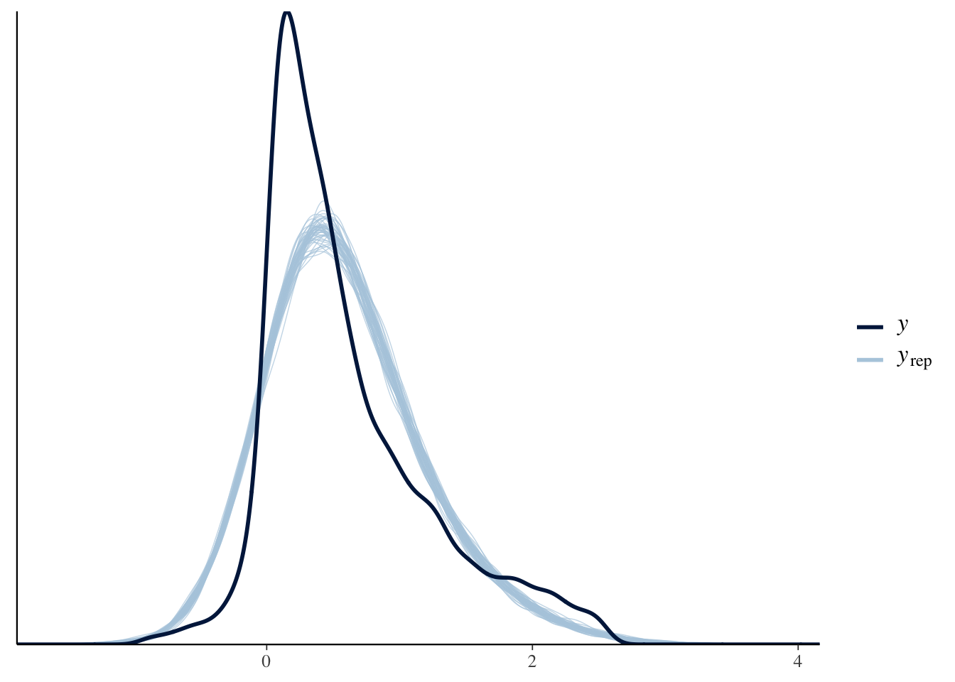
pp_check(Diff_inter_slope_train)
The model did an okay job modeling the true structure of the data. We see that several company earnings’ on the right still seem to be causing the model some difficulties.
5.2.2 Metrics
Diff_inter_slope_metrics## MAE Within95 Within50 Within90
## 1 0.2781092 0.7931034 0.4935345 0.7262931In our model with varying intercepts and slopes the average median posterior prediction is off by 0.28 billion. Furthermore, 79.3% of the earnings next year fall within the 95% prediction intervals and 49.4% are within the 50% prediction intervals.
tidy(Diff_inter_slope_train, effects = "fixed", conf.int = TRUE, conf.level = .80)## # A tibble: 13 × 5
## term estimate std.error conf.low conf.high
## <chr> <dbl> <dbl> <dbl> <dbl>
## 1 (Intercept) 0.308 0.0555 0.236 0.378
## 2 EARNINGS_Scaled 0.547 0.0203 0.521 0.573
## 3 EARNINGS_1_YEAR_AGO 0.0408 0.00697 0.0320 0.0500
## 4 SectorConsumer Discretionary -0.0272 0.0630 -0.107 0.0536
## 5 SectorConsumer Staples 0.0583 0.0726 -0.0339 0.152
## 6 SectorEnergy 0.181 0.0794 0.0778 0.283
## 7 SectorFinancials 0.119 0.0623 0.0397 0.201
## 8 SectorHealth Care 0.000288 0.0636 -0.0801 0.0823
## 9 SectorIndustrials 0.0192 0.0619 -0.0592 0.0996
## 10 SectorInformation Technology -0.0370 0.0613 -0.116 0.0419
## 11 SectorMaterials -0.0381 0.0704 -0.128 0.0521
## 12 SectorReal Estate -0.128 0.0697 -0.217 -0.0371
## 13 SectorUtilities 0.0597 0.0685 -0.0272 0.148The impact of this year’s earnings is much stronger compared to the other variables (0.5467834739). It states that for one billion increase in earnings this year, the earnings for next year will increase by 0.5467 billions. Earnings next year also has much stronger impact than earnings 1 year ago.
About the sector, the situation is also fairly similar as companies that are in Consumer Staples, Energy, or Financials will likely to have higher next year’s earnings than the others. However, in this model, the impact of the sector is smaller than the Diff_inter_train model. The most notable negative earnings impact also comes from real estate as according to the model, company that is in real estate will see the earnings next year smaller than the baseline earnings of 0.12 billions.
tidy(Diff_inter_slope_train, effects = "ran_pars")## # A tibble: 4 × 3
## term group estimate
## <chr> <chr> <dbl>
## 1 sd_(Intercept).COMPANY COMPANY 0.285
## 2 sd_EARNINGS_Scaled.COMPANY COMPANY 0.316
## 3 cor_(Intercept).EARNINGS_Scaled.COMPANY COMPANY -0.743
## 4 sd_Observation.Residual Residual 0.353The standard deviation \(\sigma_1\) in the Earnings scaled coefficient (\(\beta_{1j}\)) is likely to be around 0.31 billion per year. It refers that the standard deviation of the random slope for the Earnings coefficient is 0.31 billion dollars, which is a fairly high number.
For \(\sigma_y\), an individual Company’s net earnings next year tend to deviate from their own mean model by 0.35 billion.
There is a semi strong correlation between the Company Specific \(\beta_{0j}\) and \(\beta_{1j}\) parameters of -0.74. It seems that company’s with initial earnings will tend to experience a decrease in earnings compared to their previous years.
5.3 Summary
Our model demonstrates that future earnings are somewhat dependent on the specific company and their current and previous earnings. It also demonstrates that there are tons of other external factors that make earnings volatile from year to year, adding uncertainty into the model. The average posterior prediction for future earnings is 0.28 billion off from the true earnings that year. Furthermore, 79.3% of the earnings next year fall within the 95% prediction intervals and 49.4% are within the 50% prediction intervals. This model was the best of the ones we explored during this project, however its accuracy suffered due to the differences in companies and volatile earnings.
Pros: Our pro of our model is that we are able to have companies gain information from other companies. We can also model and edit parameter information regarding earnings between companies and within companies.
Cons: In our model, we assume earnings are indpendent of earnings in the past. However, bayes forcast is able to model soley based off past patterns and trends.